
Simulating Swift data with XSPEC
The ability to analyze spectral data from the three Swift instruments simultaneously and with consistent methodology is clearly a mission requirement. Given the historical approach of high energy astronomy to maintain separate source data and calibration files during analysis, the most flexible approach has been to write a UVOT data format that conforms to high energy software requirements. However, note that UVOT spectral data formats will also be compatible with more traditional software packages such as iraf.
This page provides step by step instructions for simulating BAT, XRT, and UVOT data with the XSPEC software package. More information about simulating BAT spectra is available on the Simulating BAT Spectra page. Under the assumption that high energy astronomers have some familarity with XSPEC, these instructions are biased towards, but not exclusive to, the analysis of UVOT data. It is expected that the software will be new to some optical afterglow researchers, while the application of XSPEC in the analysis of optical and UV data may be a novelty to many gamma-ray and X-ray researchers. The approach is, however, generic to the spectral analysis of data from all three instruments.
Before continuing, download the required calibration files to a single local directory. Please note that spectral files can also be generated using the WWW inteface webspec, while, if count rates are the only purpose of your feasibility study, pimms is the webtool of choice.
Here is a list of required reading (1), including the XSPEC User Manual and installation instructions, and useful secondary material (2):
| 1 | Required calibration files: ARFs, RMFs and RSPs |
| 1 | XSPEC: Download instructions, installation and user manual |
| 2 | The HEASARC spectral file format |
| 2 | ARF and RMF file formats |
| 2 | The WWW XSPEC interface webspec |
| 2 | The count rate simulation tool pimms |
1. Simulating spectra
The steps in this example generate spectral data for the BAT, XRT and UVOT grism filters. Red text designates characters typed by you. Green text desginates screen messages from the package.- Execute the shell script that initialises XSPEC on your local
machine by typing on the command line (where ${HEADAS} is the path to
shell script):
source ${HEADAS}/headas-init.csh
- cd to your local directory containing the ARF, RMF and RSP
files.
- Begin your XSPEC session by typing on the command line:
xspec
The following information, which will vary depending on which version of XSPEC you have installed, will be printed to your screen:
XSPEC version: 12.3.1ao Build Date/time: Mon Nov 19 15:40:01 2007 The details of the welcome message will depend on which version of XSPEC you are running, and when it was installed on your machine. Extensive on-line help is available typing: help or: ? at any time when you are given the XSPEC command prompt. The following example is specific to XSPEC 12.
- Open a plotting window, in this case, an xwindow:
XSPEC12>cpd /xw
- Build a spectral model. For this example we will use a simple
power law with an exponential high enery cutoff and an additional
power law at the highest energies. This appears to be an appropriate
model for prompt gamma ray bursts at high energies (Band
et al. 1993), although it is not appropriate for the afterglow
epoch. A full list of spectral models is availble by typing help model, but the one we are currently interested
in is constructed by typing:
XSPEC12>model grbm
The package will then prompt the user for values for each fit parameter, in this case there are four of them in this order, the low-energy powerlaw exponent (-1), the high energy powerlaw exponent (-2), the cutoff energy (150 keV) and the normalization (1):
1:grbm:alpha>-1
2:grbm:beta>-2
3:grbm:tem>150
4:grbm:norm>1
- Now we will add a component to the model to represent intrinsic
hydrogen absorption from the host galaxy. In this case we need to
adopt a redshift which we take as
z = 0.1685, the redshift of GRB 030329. 'addc 1' defines the position in the model where the new component is placed. In this case the new component is added before the first component of the current model. We will assume that the column density is NH = 5 x 1019 cm-2. The nH parameter is entered in units of 1022 atoms cm-2.XSPEC12>addc 1 zphabs
1:zphabs:nH>0.005
2:zphabs:redshift>0.1685
- Finally we add Galactic absorption to the model, where
NH = 1 x 1020 cm-2. Again, the nH
parameter is entered in units of 1022 atoms
cm-2.
XSPEC12>addc 1 wabs
1:wabs:nH>0.01Note that the new model can be listed by typing show, model components can also be deleted using delc and the entire model could have been built with the one line command model wabs*zphabs*grbm.
Also note that while we do not implement it here, the redden model characterizes Galactic extinction at energies shortward of the Lyman limit and we expect it to be used extensively to model UVOT data with XSPEC. The zredden model should be used to model extinction (with a Galactic reddening law) in the host galaxy. Alternative reddening laws are available using the zdust model.
- We're going to renormalize this spectrum appropriately to model
GRB 030329. By extrapolation, the XMM-Newton and RXTE study by Tiengo et al. (2003)
infers that the 2-10 keV afterglow flux was between 10-8
and 10-9 erg s-1 cm-2 during the
first hour after the burst. By typing the following:
XSPEC12>flux 2 10
we can find the total model flux between 2 and 10 keV. Therefore the model normalization has to be multiplied appoximately by 1.3 x 10⁻³ to recreate XMM-Newton and RXTE flux this across the Swift instruments. The newpar command is used to change the values of model parameters. In this case we want to multiply the normalization (parameter 7) by 1.3 x 10-3.
XSPEC12>newpar 7 0.0013
- Based on this model we need to generate fake data for each
instrument. Instructions for generating a fake BAT spectrum are
given on the Simulating BAT Spectra page.
- The fake data for the XRT and UVOT are generated using the
specrtral calibration files for each instrument and the command:
XSPEC12>fakeit none
For fake spectrum #1 response file is needed: ugrism.rsp
...and ancillary file: none
Use counting statistics in creating fake data? (y)y
Input optional fake file prefix:
Fake data filename (ugrism.fak): ugrism.fak
Exposure time, correction norm (1.00000, 1.00000): 3500 1Note that the name of the UVOT UV grism .rsp file should be changed to match the file downloaded from here. No ancillary response file (ARF) is required in this case because a RSP file was provided for the response file. However if an RMF file is provided instead (as is the case for the XRT calibration data), an ARF file is always required to provide the correct effective area for each instrument and/or filter.. If counting statistics are used, the spectra will be randomized according to the count rate of each channel. In this example we chose an exposure of 3500 s, i.e. ∼1 hr of accumulated exposures since the burst trigger.
In order to generate fake data for the next instrument we need to clear the UVOT UV grism data from XSPEC. This is done by: XSPEC12>data none
The fakeit none and data none step can be repeated using the XRT and UVOT optical grism. When you are done you should have four simulated data files: bat.fak, xrt.fak, ugrism.fak and vgrism.fak. Note that the data none command must be used after each fake spectrum is created except the final fakeit none command. - Now that the fake data has been created load all four spectral
data files into XSPEC. The names of the corresponding calibration
files are stored in the FITS headers of the fake data files. These
calibration files are automatically read when the fake data files are
read. In this example we are reading all four fake data sets into
data group #1. The spectrum 1 is the BAT data, spectrum 2 is the XRT
data, spectrum 3 is the UVOT ultraviolet grism data, and spectum 4 is
the UVOT visual grism data.
XSPEC>data 1:1 bat.fak 1:2 xrt.fak 1:3 ugrism.fak 1:4 vgrism.fak
Now, we want to plot the model and the fake data. XSPEC>setplot energy - Ignore specific channels in the response matrices for subsequent
plotting and analysis:
XSPEC>ignore 1:0.-15.,400.-** 2:0.-0.1,12.-**
In this case we are telling XSPEC to ignore channels in spectrum 1 (BAT) with energies between 1.0 and 15.0 keV and 400 keV and above (1:0.-15.,400.-**), and channels in spectrum 2 (XRT) with energies between 0.0 and 0.1 keV and 12.0 keV and above (0.-0.1,12.-**). The units specified are those of the energy class just specified with the setplot command and specifying the decimal point is crucial in this instance.
- Rebin the data so that channels with low count rates are binned
with neighbouring channels. In this case the channels are rebinned so
that the minimum significance in each bin is 5-sigma and the maximum
number of bins that can be combined is 1000.
XSPEC>setplot rebin 5 1000
- The effective areas of the instruments can be plotted with the
command:
XSPEC>plot efficien
where the result will be similar to what is shown in Fig 1.1. The figure in your plotting window can be beautified to your own taste using the iplot function and then the PLT command language.
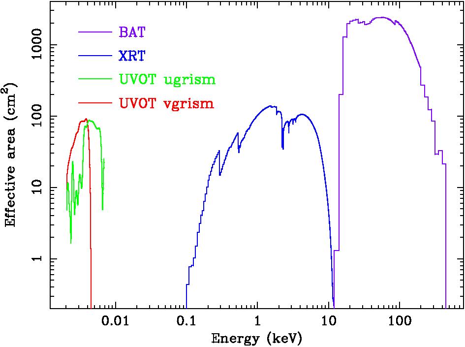
Figure 1.1: Effective areas of BAT, XRT and UVOT grism instruments.
- A logarithmic count rate spectra and χ2 fitting
statistic (Fig 1.2) can be plotted thus:
XSPEC>plot ldata delchi
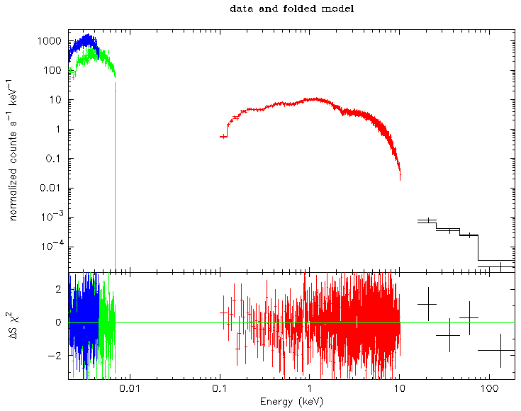
Figure 1.2: Count rate spectrum of simulated BAT, XRT and UVOT grism data. A χ2 comparison between data and model is illustrated in the lower panel.
- A νFν version of the spectrum (Fig. 1.3) can
be obtained using:
XSPEC>plot eufspec
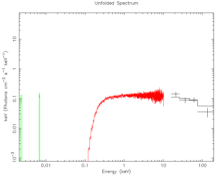
Figure 1.3: νFν spectrum of simulated BAT, XRT and UVOT grism data. The black line is the model, blue points the data.
- To make things a bit more interesting we can change the redshift
of the model:
XSPEC>newpar 3 3.0
and rerun fakit to alter the data accordingly. Since all the response matrices are already loaded, this task is now less onerous:
XSPEC>fakeit none
For fake spectrum #1 response file is needed: swbresponse20030101v007.rsp
... and ancillary file:
Use counting statistics in creating fake data? (y)
Input optional fake file prefix:
Fake data file name (bat.fak.fak):bat.fak
File bat.fak exists - overwrite? (yY/) or (nN)
Exposure time, correction norm (1.00000, 1.00000): 3500 1
Fake data file name (xrt.fak.fak):xrt.fak
File xrt.fak exists - overwrite? (yY/) or (nN)
Exposure time, correction norm (3500.00, -1.00000): 3500 1
Fake data file name (ugrism.fak.fak): ugrism.fak
File ugrism.fak exists - overwrite? (yY/) or (nN)
Exposure time, correction norm (3500.00, -1.00000): 3500 1
Fake data file name (vgrism.fak.fak): vgrism.fak
File vgrism.fak exists - overwrite? (yY/) or (nN)
Exposure time, correction norm (3500.00, -1.00000): 3500 1Again, we want to ignore some channels and rebin the data. XSPEC>ignore 1:0.-15.,400.-** 2:0.-0.1,12.-**
XSPEC>setplot rebin 5 1000
The redshift parameter can be fit after unfreezing the parameter in the model. XSPEC>thaw 3
Fit the model to the data and specify that no more than 100 fitting iterations should be carried out. XSPEC>fit 100
The data and model are plotted in Fig. 1.4. Here we chose to plot the UVOT spectra in wavelength units by typing:XSPEC>setplot wave
We want to ignore the XRT data, which has wavelengths significantly less than 1000 Angstrom. XSPEC>ignore **-1000Here we pass two commands to the plotting facility. The first is wind all which tells plot to apply the following command to all windows. The second is log x off which turns off the logarithmic scale on the X axis. XSPEC>setplot comm wind all
XSPEC>setplot comm log x off
XSPEC>plot ldata delchi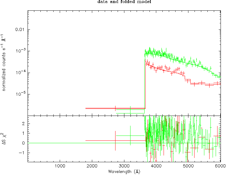
Figure 1.4: Grism spectra simulated from an identical model which has been redshifted to z = 3.0 The Lyman limit of the host galaxy now resides in the UVOT band, enabling a redshift determination.
Note, of course, that this is a slightly cheeky example since, by relocating GRB030329 to z = 3, the distance increases by a factor 18 and the source flux should decrease by factor 324!!
2. Simulating broad band filters
This example uses the same model as above to simulate data from the broad band filters UVW2, UVM2, UVW1, U, B and V. The response matrices in this case yield one data point per filter. Therefore, the broad band filters must be combined with other filters or instruments in order to reveal spectral information.- After setting up and starting your xspec environment, build the
model. This model is the same as was used in the previous example,
but here we are building it all at once.
XSPEC>model wabs*zphabs*grbm
1:wabs:nH>0.01
2:zphabs:nH>0.005
3:zphabs:redshift>0.1685
4:grbm:alpha>-1
5:grbm:beta>-2
6:grbm:tem>150
7:grbm:norm>0.0013 - simulate UVW2 data from this model:
XSPEC>fakeit none
For fake spectrum #1 response file is needed: swuw2_20041120v104.rsp
... and ancillary file:
Use counting statistics in creating fake data? (y):
Input optional fake file prefix:
Fake data filename (swuw2_20041120v104.fak): uvw2.fakExposure time, correction norm (1.00000, 1.0000): 3500 1
XSPEC12>data none
and repeat for the filters UVM2, UVW1, U, B and V. Do not forget to use data none after each fakeit none command.
- Load all 6 response matrices and simulated data files into the
package:
XSPEC>data 1:1 uvw2.fak 1:2 uvm2.fak 1:3 uvw1.fak 1:4 u.fak 1:5 b.fak 1:6 v.fak
- Open a plotting window and set the plotting units to a wavelength
scale:
XSPEC>cpd /xw
XSPEC>setplot wave
XSPEC>setplot command window all
XSPEC>setplot command log x off - Plot the filter effective areas:
XSPEC>plot efficien
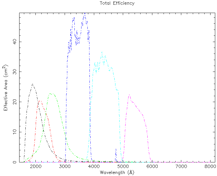
Figure 2.1: Effective areas of the UVW2, UVM2, UVM1, U, B and V UVOT filters.
- Plot the count rate spectrum, with model and
χ2:
XSPEC>plot ldata delchi
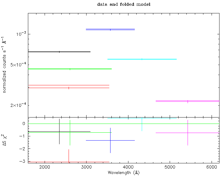
Figure 2.2: Simulated count rate spectrum, model and χ2 from the UVW2, UVM2, UVM1, U, B and V UVOT filters.
- If we now repeat this exercise after moving the model to a
redshift of z = 3.0:
XSPEC>newpar 3 3.0
XSPEC>fake none
For fake spectrum #1 response file is needed: swuw2_20041120v104.rsp.rsp
... and ancillary response file:
Use counting statistics in creating fake data? (y)
Input optional fake file prefix (max 8 chars):
Fake data file name (uvw2.fak.fak): uvw2.fak
File uvw2.fak exists - overwrite? (yY/) or (nN):Exposure time, correction norm (1.00000, 1.00000): 3500 1
Fake data file name (uvm2.fak.fak): uvm2.fak
File uvm2.fak exists - overwrite? (yY/) or (nN):Exposure time, correction norm (3500.00, 1.00000): 3500 1
Fake data file name (uvw1.fak.fak): uvw1.fak
File uvw1.fak exists - overwrite? (yY/) or (nN):Exposure time, correction norm (3500.00, 1.00000): 3500 1
Fake data file name (u.fak.fak): u.fak
File u.fak exists - overwrite? (yY/) or (nN):Exposure time, correction norm (3500.00, 1.00000): 3500 1
Fake data file name (b.fak.fak): b.fak
File b.fak exists - overwrite? (yY/) or (nN):Exposure time, correction norm (3500.00, 1.00000): 3500 1
Fake data file name (v.fak.fak): v.fak
File v.fak exists - overwrite? (yY/) or (nN):Exposure time, correction norm (3500.00, 1.00000): 3500 1
We arrive at the following spectrum plot:
plot ldata delchi
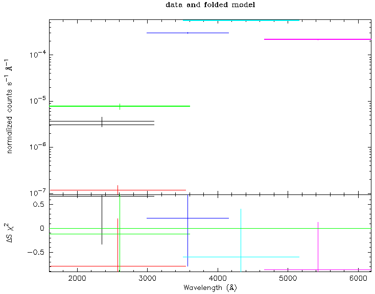
Figure 2.2: Count rate spectrum, model and χ2 from the UVW2, UVM2, UVM1, U, B and V UVOT filters after the model has been moved to a redshift of z = 3.0
The UVW2, UVM2 and UVW1 count rates are reduced significantly compared to the z = 0.1685 model, whereas the B and V count rates are largely unchanged. We can infer with this data that the Lyman break occurs somewhere in the U band. - In principle, if the intrinsic spectrum is well constrained, the
broad band filters can provide excellent constraints for z. Fitting
for z, as follows:
XSPEC>thaw 3
Freeze model parameters 1, 2, 5, and 6 (Galactic nH, host galaxy nH, beta, and temperature). XSPEC>freeze 1,2,5,6
XSPEC>fitwe obtain z = 3.997 ± 0.009 with 90 percent confidence. Of course, this requires BAT and XRT measurements in order to assume a spectral shape. However we must also consider extinction and the strengh of the Lyman series and other possible line features close to the break in order before making a redshift measurement with the broad band filters. Consequently, for bright sources, the grism data is a superior resource. For fainter sources, of which the grism filters are not useful and the intrinsic spectrum is more uncertain, the shape of the spectrum is less of an issue because event statistics yield a poorer quality fit. For example if we reduce the flux of the source appropriately for a redshift of z = 3.0:
XSPEC>newpar 7 4.E-6
XSPEC>fakeit none etc...
XSPEC>fit
XSPEC>error 3Our solution is z = 3.087 ± 0.123 with 90 percent confidence. Clearly the details of the spectral shape near the Lyman limit are less of an issue in these faint cases.
- Note that the UVOT bandpass extends down to approximately 1700 Å and, consequently, the Lyman limit cannot be detected by UVOT at redshifts of approximately z < 1. However an accurate redshift may be determined possibly from narrow lines, perhaps in the grism or XRT data (Reeves et al. 2002).
3. Simulating XRT spectra
As a final exercise we look at a model of an extragalactic source that has power law spectrum with two emission lines superimposed. We assume both Galactic absorption and absorption in the source.- Build the model and create a spectrum:
XSPEC>mo wabs*zphabs*(powerlaw+zgauss+zgauss)*wabs
1:wabs:nH>0.01
2:zphabs:nH>0.005
3:zphabs:redshift>0.0685
4:powerlaw:PhoIndex>-2
5:powerlaw:norm>0.126
6:zgauss:LineE>1.35
7:zgauss:Sigma>1.0000E-02
8:zgauss:redshift>0.0685
9:zgauss:norm>3.6900E-02
10:zgauss:LineE>2.01
11:zgauss:Sigma>1.0000E-02
12:zgauss:redshift>0.0685
13:zgauss:norm>3.3500E-02
Now, we want to fix the three redshifts to the same value so that they vary together and not independently. XSPEC>newpar 8 = 3
XSPEC>newpar 12 = 3
Next, generate the fake data. XSPEC>fakeit none
For fake spectrum #1 response file is needed: swuxpc1to12s0_20010101v010.rmf.rsp
... and ancillary response file: swxpc0to12s0_20010101v010.arf Use counting statistics in creating fake data? (y):
Input optional fake file prefix:
Fake data file name (swxpc0to12s0_20010101v010.fak): xrt.fak
Exposure time, correction norm (1.00000, 1.00000):3500 1
Tell XSPEC to ignore data outside its usual energy range (0.1 to 12 keV). XSPEC>ignore 0.0-0.1,12.0-**
XSPEC>setplot rebin 5 1000
XSPEC>cpd /xwXSPEC>plot ldata del
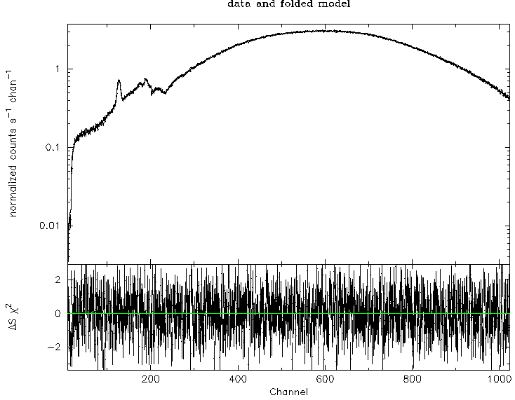
Figure 2.2: Simulated count rate spectrum, model and χ2 for a bright source with the XRT.
- Two emission lines, between channel 100 and 200, are clearly
resolved in this instance. The uncertainty for the redshift is found
by:
XSPEC>thaw 3
XSPEC>fit
XSPEC>error 3
The redshift is found be between z = 0.059 and 0.078 with 90 percent confidence. The fitted photon index of the power law spectrum is -1.999 +/- 0.002. The fitted absorption in the source is (1.100 +/- 0.198) x 1022 atoms cm-2.
- After setting up and starting your xspec environment, build the
model. This model is the same as was used in the previous example,
but here we are building it all at once.

- Curator: J.D. Myers
- NASA Official & Swift PI: Brad Cenko
- PAO Contact: Francis Reddy
- Questions/Comments/Feedback
- › Privacy Policy and Important Notices
- › Accessibility
- › Contact NASA
- › Page Last Updated: Tue, Mar 27, 2012