Broad-Band Spectral Fitting

Overview:

This thread gives a description how you can perform a broad-band (opt/UV/X-ray) spectral fitting to 6-filter UVOT and XRT data to obtain the spectral energy distribution (SED) of your source of interest.

Read this thread if you want to: Perform a broad-band spectral fitting to UVOT and XRT data.

Last update: Dec 4, 2006

In this thread we describe how to

1) extract a spectrum from UVOT data,
2) shift the count rates of the spectrum to a common epoch,
3) extract an XRT X-ray spectrum, and
4) perform a joint spectral fitting of the UVOT and XRT data.

The example below uses data obtained on GRB 050525 (sequence 00130088000).

1) Extract Spectrum from UVOT Data:

You can use individual UVOT images or co-add individual image extensions to one image per filter to increase the photon statistics:

uvotimsum sw00130088000uvv_sk.img uvv_sum.fits chatter=1
uvotimsum sw00130088000ubb_sk.img ubb_sum.fits chatter=1
uvotimsum sw00130088000uuu_sk.img uuu_sum.fits chatter=1
uvotimsum sw00130088000uw1_sk.img uw1_sum.fits chatter=1
uvotimsum sw00130088000um2_sk.img um2_sum.fits chatter=1
uvotimsum sw00130088000uw2_sk.img uw2_sum.fits chatter=1

Certain file extentions can be excluded from being coadded (if need) by employing the 'exclude' parameter, e.g.:

uvotimsum sw00130088000uw2_sk.img uw2_sum.fits chatter=1 exclude=1

Now load the images into DS9 and create source and background region files:

ds9 uvv_sum.fits &

The burst is located at RA = 18:32:32.6, Dec = 26:20:22.3. The source spectrum region file, 'source.reg', centered in the burst needs to be in WCS coordinates, either in degrees or in sexadesimal format:

fk5;circle(18:32:32.599,+26:20:22.27,6")

fk5;circle(278.13583,26.339519,6")

A background region file, 'back.reg', also needs to be created with DS9.

A response matrix is needed which defines the spectral properties of the data. These can be downloaded from the Swift web pages where there is one available for every lenticular UVOT filter. It is critical that the correct response matrix be used with the data (easily identified by the names of the files):

http://swift.gsfc.nasa.gov/docs/swift/proposals/swift_responses.html

Next, you can use the tool 'uvot2pha' to create a file that can be read into XSpec. Given the two region files, one containing source counts from a specific object, the other containing background counts from around that source, UVOT2PHA will extract counts from both regions accompanied by Poisson uncertainties. These four quantities will be cast into two XSpec-compatible files.

uvot2pha infile=uvv_sum.fits srcpha=v.pha bkgpha=v_bkg.pha \
srcreg=source_v.reg bkgreg=back_v.reg respfile=v.rsp clobber=y chatter=1

uvot2pha infile=ubb_sum.fits srcpha=b.pha bkgpha=b_bkg.pha \
srcreg=source_b.reg bkgreg=back_b.reg respfile=b.rsp clobber=y chatter=1

uvot2pha infile=uuu_sum.fits srcpha=u.pha bkgpha=u_bkg.pha \
srcreg=source_u.reg bkgreg=back_u.reg respfile=u.rsp clobber=y chatter=1

uvot2pha infile=uw1_sum.fits srcpha=uvw1.pha bkgpha=uvw1_bkg.pha \
srcreg=source_uvw1.reg bkgreg=back_uvw1.reg respfile=uvw1.rsp clobber=y chatter=1

uvot2pha infile=um2_sum.fits srcpha=uvm2.pha bkgpha=uvm2_bkg.pha \
srcreg=source_uvm2.reg bkgreg=back_uvm2.reg respfile=uvm2.rsp clobber=y chatter=1

uvot2pha infile=uw2_sum.fits srcpha=uvw2.pha bkgpha=uvw2_bkg.pha \
srcreg=source_uvw2.reg bkgreg=back_uvw2.reg respfile=uvw2.rsp clobber=y chatter=1

2) Correct for a Temporal Variation/Decay of the Source:

It is important to note that some astronomical objects, such as GRBs and supernovae, vary in flux on relatively short-term time scales. In order to do a correct broad-band spectral fitting, the variability of the source therefore has to be taken into account. There are two methods you could chose which are described below. We leave it to the user which method is employed (this is where the 'art' of being a scientist comes in).

1) Select data from simultaneous epochs:

Select your epoch of interest for which you want well sampled data in the X-ray and UV/optical. For X-ray data you can extract the time-interval of interest within 'xselect' and produce a spectrum that can be read into XSpec. For the UVOT you want to obtain the exposures in each filter that correspond to the epoch of intestest and co-add them into one image per filter.

2) Fit data to get an SED at an instantaneous epoch:

For this method you need to fit each light curve individually and use the fit to determine the corresponding count rate at the epoch of interest. In the case of the UVOT filters, to be accurate, you want to perform a simultaneous fit to get an accurate measure of the decay rate. You then re-fit your data filter by filter, fixing the decay slope in each case to the best-fit value determined earlier. If you want to check if your source shows evidence for a color evolution, you have to do this for multiple epochs. Once you have derived count rates, you then produce your spectral files as described below, within 'xselect' and using 'uvot2pha'. You then need to update the 'EXPOSURE' header keyword appropriately so that the count rate will be the one that you measured in your fits.

In detail, these are the steps that have to be performed to shift a UVOT .pha file to common epoch:

Input:

source.pha file
background.pha file

1) Scale the background counts (or count rate) so that it has the same area as the source counts.

2) Subtract the scaled background counts from the source counts.

3) Compute the counts at the time of the common epoch using the observed decay rate of the afterglow. For a power-law decay the relationship is

   counts_common_epoch = count_original * ( t_common_epoch / t_original )^alpha

   where t is the time since the BAT trigger.

4) Add the background to the shifted counts to get the total counts at the common epoch.

5) Propagate the errors.

   sp = statistical error in shifted counts
   s = statistical error in original counts
   sb = statistical error in background counts
   f = ( t_common_epoch / t_original )^alpha
   g = area of source region / area of background region

   sp = SQRT([f * s]² + [f * g * sb]²)

3) Extract Spectrum from XRT Data:

Load the cleaned XRT photon-counting events file into ds9

ds9 sw00130088000xpcw4po_cl.evt

and create a region file centered in the X-ray sources, as well as a background region file. In our case, we chose a circular region file in WCS sky coordinates, centered on the source, and an annulus around the source as background region file:

source_xrt.reg:

fk5;circle(278.13583,26.33951,47")

choosing a circle of radius 20 pixel (47 arcsec) which corresponds to the 90% encircled energy radius at 1.5 keV. The background region files has the form:

back_xrt.reg:

fk5;annulus(278.13571,26.339051,75",150")

'xselect' can be used to extract counts from the events file using a spatial filtering with the region files, and writing them to spectral files suitable for XSpec:

xselect

> Enter session name
> [xsel]xsel:SUZAKU
> read events sw00130088000xpcw4po_cl.evt
> Enter the Event file dir >[./]Got new mission: SWIFT
> Reset the mission ? >[yes]

Notes: XSELECT set up for SWIFT
Time keyword is TIME in units of s
Default timing binsize = 5.0000

Setting...
Image keywords = X Y with binning = 1
WMAP keywords = X Y with binning = 1
Energy keyword = PI with binning = 1

Getting Min and Max for Energy Column...
Got min and max for PI: 0 1023

Got the minimum time resolution of the read data: 2.5073
MJDREF = 5.1910000742870E+04 with TIMESYS = TT
Number of files read in: 1

Observation Catalogue:

Data Directory is: /namibia/00130088000/xrt/event/ HK Directory is: /namibia/GRB050525/00130088000/xrt/event/

OBJECT OBS_ID DATE-OBS DATAMODE
1 GRB050525 00130088000 2005-05-25T PHOTON

xsel:SWIFT-XRT-PHOTON > set image sky
xsel:SWIFT-XRT-PHOTON > filter region source_xrt.reg
xsel:SWIFT-XRT-PHOTON > extract spectrum

extractor v4.67 11 Jul 2006
Getting FITS WCS Keywords
Doing file: /namibia/00130088000/xrt/event/sw00130088000xpcw4po_cl.evt
100% completed
Total Good Bad: Region Time Phase Grade Cut
3269 609 2660 0 0 0 0
Grand Total Good Bad: Region Time Phase Grade Cut
3269 609 2660 0 0 0 0
in 5755.9 seconds
Spectrum has 609 counts for .1058 counts/sec
written the PHA data Extension

xsel:SWIFT-XRT-PHOTON

> save spectrum xrt.pha

Wrote spectrum to xrt.pha

Next, do the same for the background region file and create a background spectrum, xrt_back.pha.

Now the response matrix and ancillary response file need to be created using xrtmkarf or downloaded from the Swift calibration site. In this example, we write the headers for the generic response files into the XRT spectrum:

xrtmkarf
Name of the input PHA FITS file[] xrt.pha
PSF correction active?(yes/no)[yes]
Name of the output ARF FITS file[] xrt.arf
Source X coordinate (SKY for PC and WT modes, DET for PD mode):[-1] 278.13583
Source Y coordinate (SKY for PC and WT modes, DET for PD mode):[-1] 26.339519

grppha
Please enter PHA filename[xrt.pha] xrt.pha
Please enter output filename[xrt.pha] xrt.pi
GRPPHA[] chkey RESPFILE swxpc0to12_20010101v008.rmf
GRPPHA[] chkey ANCRFILE xrt.arf
GRPPHA[] chkey BACKFILE xrt_back.pha
GRPPHA[] exit

written the PHA data Extension
exiting, changes written to file : xrt.pi
grppha 3.0.0 completed successfully

4) Joint Spectral Fitting of UVOT and XRT Data:

Start an XSpec session, read in the UVOT and XRT data, ignore energy channels outside the energy range of the instrument, and fit the data:

XSPEC>cpd /xw
XSPEC>data 1:1 v.pha 1:2 b.pha 1:3 u.pha 1:4 uvw1.pha 1:5 uvm2.pha 1:6 uvw2.pha 2:1 xrt.pha
XSPEC>setpl en
XSPEC>ignore bad
XSPEC>ignore 0.0-0.0005,7.0-**
XSPEC>plot ldata
XSPEC>mo zwabs*power+wabs*power
XSPEC>fit

Note that we read the XRT spectral file seperately (data 2:1), which allows that the normlization can be fitted.
After you found a satisfying fit to the data, make a nice plot in IPLOT:

XSPEC> iplot

PLT> plot
PLT> label top
PLT> label file
PLT> time off
PLT> lwidth=2
PLT> la x Channel Energy (keV)
PLT> la y Counts s\u-1\d keV\u-1\d
PLT> plot

and create a postscript file:

PLT> hardcopy GRB050525.ps/cps

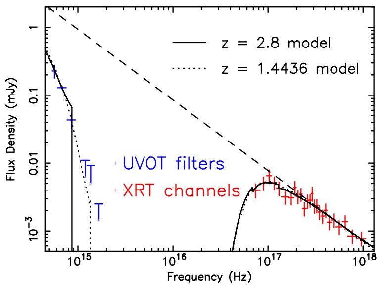
The output of the broad-band spectral fitting is shown in the figure below. UVOT data are given in blue, XRT in red.