
Notes for observing with the UVOT UV Grism
Last updated: 16-Sep-2009: Updated software statusThe UVOT UV grism can provide 1700 - 2900 Å spectra of modest S/N and spectral resolution R ~ 150 for stars in the magnitude range 11-15. The UV grism spectrum actually extends longward of 2900 Å but these longer wavelength regions can be confused by overlap from UV second-order light. Note that the V grism is sensitive down to 2800 Å, and is actually more sensitive than the UV grism for the longest wavelength UV light (2900 -3200 Å).
The wavelength calibration of the UV grism has been difficult because the spectra show a curvature and sensitivity that varies with detector position. Because the UVOT pointing is only repeatable to within a few arcseconds (even with a slew in place), there are variations even within consecutive calibration exposures. These variations are minimized by placing the target in the lower half of the detector, but such offsets are not possible if simultaneous XRT spectra are desired.
The following decisions need to be made when observing with the UV grism:
- Slew in place?: The pointing accuracy after an initial slew may be only 1 or 2 arcminutes. This uncertainty is not significant for GRB followups with direct images, but can critically affect the calibration of the UV grism data, since there are large wavelength and sensitivity changes across the detector. The use of a second slew after the arrival at the target (a "slew in place") can reduce the pointing uncertainty to a few arcseconds. However, if one is primarily interested in XRT data then one might not want to spend the extra ~3 minutes required to improve the grism observation by taking a slew in place. Note that one often one tries to avoid observing with the grism during the first few and last few minutes of an orbit anyway (because the sky background is large) so the use of a slew in place does not affect the prime grism science time.
- Clocked or Nominal
Mode?:
Zero-order spectra only appear in the area covered by the grism,
whereas
first-order spectra can be dispersed off the edge of the grism. Thus,
in principle, the use of clocked mode can minimize the contamination of
first-order spectra by unrelated zeroth-order images. Unfortunately,
for the UV grism the default clocking is insufficient to perform this
separation for the UV first-order spectrum. However, clocked mode
remains
useful because it suppresses the total sky flux, and for that reason must be used
in crowded fields
(e.g. low Galactic latitudes). Clocked mode also has slightly better
sensitivity (see below) and smaller spatial variations in wavelengths
and sensitivity. One disadvantage of clocked mode is that it introduces
vignetting and so spectra are retrieved over a smaller field, which may
be important for extended sources or if a slew in place is not used.
For sparse fields, the choice between clocked and nominal mode is often
decided by which one gives a better roll angle for a particular
observing
date.
- Roll Angle: The contamination of grism spectra by zero and first order of unrelated sources depends on the roll angle of the observation. An IDL grism simulator is available at http://idlastro.gsfc.nasa.gov/ftp/landsman/simgrism/ which displays a DSS image with simulated dispersed spectra for a given roll angle. (This software can be run under the IDL virtual machine, without an IDL license.) For a given observing time, the planners have very limited flexibility in choosing the roll angle. However, the simulator can be used to select a range of good observing dates or to choose between clocked and nominal model.
- Exposure time:
The June 2006 effective area for the U grism in the nominal and clocked
modes at the target position is given in the table below. Note that
this
effective area is for computing the count rate integrated perpendicular
to the dispersion, and that the dispersion varies from about 2.0
Å/pixel
near 1800 Å to about 3.5 Å/pixel near 3000 Å. The
"Cts/s" column gives
the predicted counts/s (per pixel integrated perpendicular to the
dispersion) for a source wtih a flat spectrum of 10^(-13) erg cm(-2)
s(-1) Å(-1).
| Wavelength |
Nominal |
Clocked |
||
|---|---|---|---|---|
| (Å) |
cm^2 |
Cts/s |
cm^2 |
Cts/s |
| 1700 |
2.1 |
0.032 |
1.6 |
0.021 |
| 1800 |
3.4 |
0.063 |
3.5 |
0.065 |
| 1900 |
5.3 |
0.11 |
5.9 |
0.13 |
| 2000 |
6.9 |
0.17 |
8.3 |
0.20 |
| 2100 |
9.0 |
0.24 |
9.9 |
0.27 |
| 2200 |
10.7 |
0.32 |
11.4 |
0.35 |
| 2300 |
11.4 |
0.38 |
13.0 |
0.43 |
| 2400 |
12.0 |
0.43 |
14.4 |
0.52 |
| 2500 |
12.3 |
0.48 |
14.8 |
0.58 |
| 2600 |
12.5 |
0.52 |
14.8 |
0.62 |
| 2700 |
13.3 |
0.59 |
13.9 |
0.62 |
| 2800 |
13.3 |
0.63 |
12.1 |
0.57 |
| 2900 |
11.7 |
0.58 |
10.5 |
0.52 |
- Background Count Rate: Observations of faint sources are dominated by the background count rate, which must be considered when predicting the expected S/N. The sky background on a grism image increases with decreasing Galactic latitude, ecliptic latitude, Sun angle, and Earth limb angle. The background counts per second in a 13 pixel extraction slit roughly varies from about 0.4 cps at low Galactic latitude to about 0.2 cps at high Galactic latitude. (A 13 pixel extraction slit is roughly the smallest slit size that does not significantly reduce the source count rate.) Consider the computation of the S/N at 2500 Å in a 2000s exposure of a high Galactic latitude source with a monochromatic flux of 10^(-14) erg cm(-2) s(-1) Å(-1) in the nominal grism mode. From the table above the expected source rate is 0.048 cps. The S/N then is S/sqrt(S+B) = (2000*0.048)/sqrt(2000*(0.2 +0.048)) = 4.3. The actual S/N will be somewhat lower because the background includes non-random noise due to the presence of faint stars and first-order spectra.
Effective Area
The effective area for all four grism modes is plotted below. Note that although the UV grism can record a visible spectrum, the sensitivity is less than half that of the V grism, and can suffer significant contamination from second-order UV light.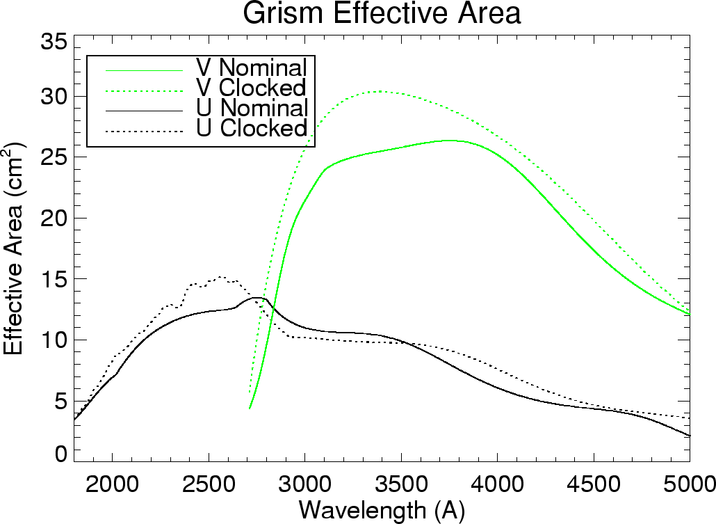
Caveats
Some considerations to be aware of when using the UV grism.- A single grism spectrum shows a fixed pattern noise
that is
only partially suppressed by applying a mod-8 correction. It may be
useful to combine
spectra with shifted zero order positions to further suppress this
fixed-pattern noise.
- There is currently no method to correct for
coincidence
losses of bright spectra. Co-I losses will begin to be significant at
2800 Å at
a flux of approximately 10^(-12) erg cm^-2 s^-1
Å^-1.
- The wavelength anchor point is defined by the centroid of the zeroth order. However, because the zeroth order is dispersed the position of the anchor point may vary with spectral shape. In addition, mod-8 noise may shift the position of the centroid. Finally, the zeroth order (which contains both UV and visible light) is often saturated. So there may be a zero point shift of up to 3-4 pixels ( 10 Å).
- The grism has only recently been used to study GRBs
(see Kuin
et al. 2009) , and thus until recently the
SWIFT
grism tools (e.g. uvotimgrism) have been given low
priority. A new tool uvotgraspcorr is now available
to compute an astrometric solution for grism images. This
allows the centroid of the zero order to specfied by giving the source
RA and Dec, This astrometric correction is not yet
in the UVOT pipeline, but grism users can request astrometrically
corrected images and the default extracted 1-d
spectra. A complete rewrite of the grism software
based on modeling of the grism optics should be available at the end of
2009. This new software should be especially useful
for UV observations taken without a slew in place
Example Spectra
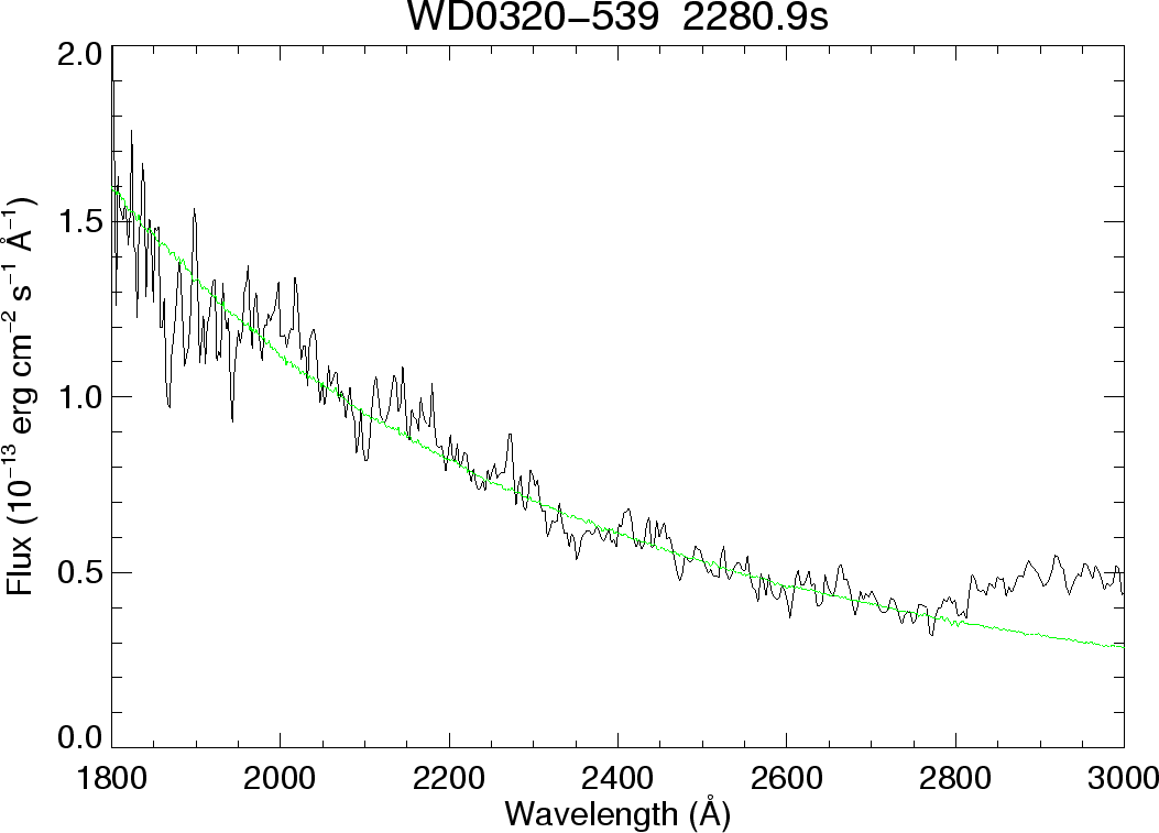
Three examples of UVOT UV grism spectra are shown below. Figure 1 shows RS Oph in outburst (V ~ 9.5) in March 2006. This spectrum shows N III] 1750 Å emission which is at the extreme wavelength limit of the UV grism sensitivity. Figure 2 is a spectrum of comet 3P/Schwassmann-Wachmann obtained in April 2006 showing CS and OH ultraviolet emission lines. Figure 3 shows a UVOT spectrum of the 14th magnitude calibration white dwarf WD0 320-539 compared with an HST spectrum (in green). For this hot source, the second-order UV light is already present at 2850 Å, as seen in the excess flux compared to the HST spectrum.Figure 1
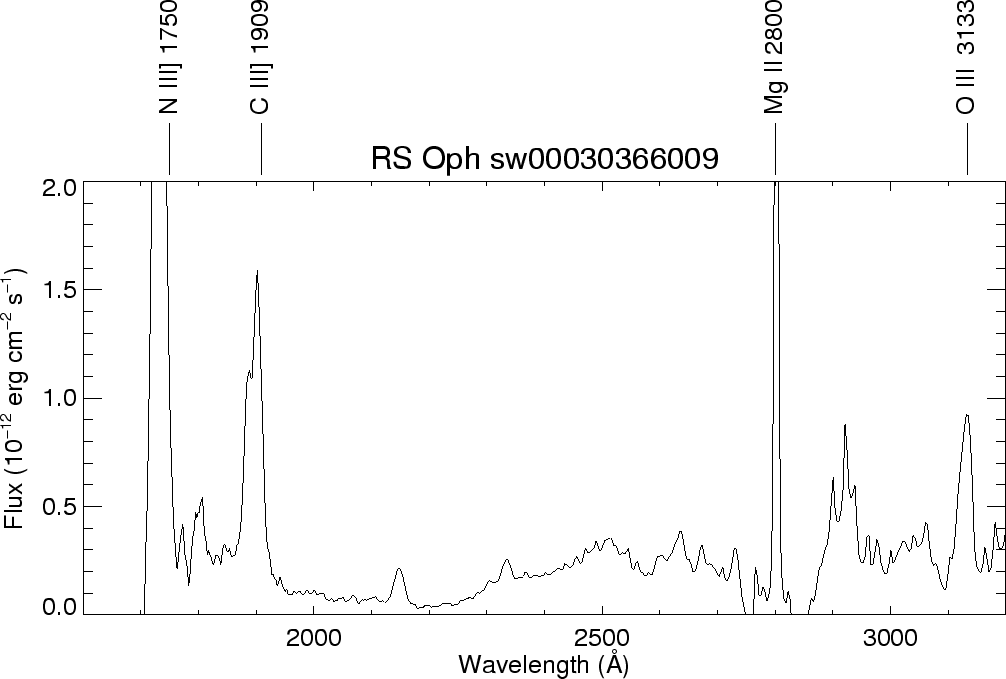
Figure 2
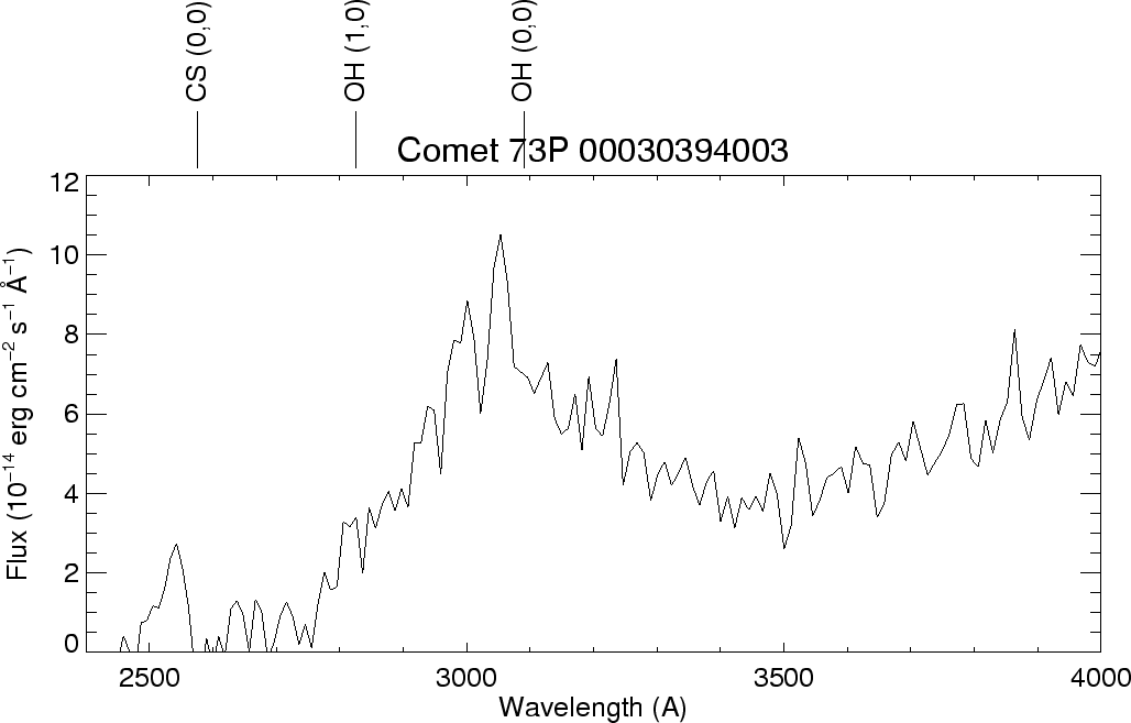
Figure 3

- Curator: J.D. Myers
- NASA Official & Swift PI: Brad Cenko
- PAO Contact: Francis Reddy
- Questions/Comments/Feedback
- › Privacy Policy and Important Notices
- › Accessibility
- › Contact NASA
- › Page Last Updated: Thu, Apr 26, 2012